exploring an oceanic time machine of modelling data via web API

Author: Iwan Cornelius

Date: 23 April 2024

the blue economy

The blue economy refers to activities that utilise and conserve ocean resources, encompassing sectors such as fisheries, aquaculture, tourism, renewable energy, shipping, and marine ecology. The integration of oceanographic data has potential to enhance the efficiency, sustainability, and safety of these activities and others like them.

what is oceanography?

Oceanography is the scientific study of the ocean and its phenomena. This field encompasses the exploration and comprehensive analysis of various aspects of the oceanic environment, including its physical, chemical, biological, and geological attributes. Oceanographers examine the properties and dynamics of ocean waters, the life that inhabits them, and the interactions between the ocean and other parts of the Earth's system, such as the atmosphere and the seafloor. Not all innovators in the blue economy are oceanographers, however, they could be engineers, entrepreneurs, environmental scientists, marine biologists, economists, policy makers, and technology developers.

software innovation in the blue economy

Innovations in software can revolutionise the blue economy by enhancing sustainability and operational efficiency sector-wide. Marine Spatial Planning (MSP) software aids in allocating marine spaces to balance economic, environmental, and social objectives, while fisheries management tools monitor fish populations and manage fishing efforts. Shipping and port management systems optimise shipping routes and port operations, reducing fuel consumption and emissions savings costs and earning carbon credits. In the realm of renewable energy, planning software requires models of ocean conditions to optimise the placement of turbines for wind, wave, and tidal energy, improving energy output and grid integration. Environmental monitoring tools use satellite imagery and sensor data to protect marine habitats and detect illegal activities, supporting conservation efforts. These software innovations ensure that marine resource management is data-driven, efficient, and environmentally responsible, supporting the sustainable growth of the blue economy.

what is the nemo model?

The NEMO (Nucleus for European Modelling of the Ocean) model is a framework for simulating and forecasting global ocean dynamics, offering access to both historical and forecast three dimensional datasets. It's a veritable ocean data time machine. These datasets include variables like temperature, salinity, currents, and biogeochemical markers such as pH, chlorophyll, and net primary production, all vital for examining the ocean's physical state and ecosystem health. Beyond scientific research, NEMO has broad applications, including but not limited to:

• Maritime Transportation: providing forecasts of ocean currents, sea surface temperatures, and wave conditions can optimise shipping routes to enhance fuel efficiency and safety.
• Fisheries and Aquaculture Management: modelling the oceanic conditions affecting fish populations can aid in sustainable fisheries management and aquaculture planning.
• Offshore Renewable Energy: simulating ocean conditions for the installation and operation of energy infrastructure like wind turbines and tidal power stations, optimising location and energy production.
• Environmental Monitoring and Protection: predicting pollutant dispersal patterns, such as oil spills or plastic debris, enables effective response strategies and marine habitat protection.

amentum scientific's ocean web api refresh

We are pleased to announce the latest update to our Ocean Web API- - now making NEMO's hindcast and forecast physical and biogeochemistry data easily accessible from any programming language that supports HTTP requests. The web API already empowers our customers to build innovative solutions like those mentioned above. With the addition of the NEMO endpoint, we look forward to empowering many more innovators by incorporating ocean data into their software innovations.

Let's take a quick look at the API's capabilities. Herein we consider a candidate shipping route between Australia and Japan, calculated by the SeaRoutes API, for a nominal departure date of 22nd April 2024. We then obtain a forecast of the ocean physical and biogeochemistry properties at each waypoint using the updated NEMO endpoint of our API, at a depth of 10 metres, and bathymetry data obtained using the existing GEBCO endpoint. Sidenote: we obtained these properties for a fixed date, we can improve accuracy by assigning correct dates to each waypoint.

Our analysis code was written in Python with help from async_api_caller: our lightweight open source package for efficient asynchronous API calls. Data wrangling is performed using the pandas package, and visualised using the plotly package. The figures below show the route and profiles of NEMO data along that.

Figure: The sample shipping route between Australian and Japanese ports.

Figure: The salinity profile along the route showing a dip at the red marker (corresponding to coordinates shown by the tooltip in the above figure).

Figure: There was no marked change in temperature at the same location as the salinity depression (red dot); however, we did see the expected decrease in sea temperatures as we approach Japan.

Figure: Remarkable fluctuations in sea depth along the route, and the variation in spatial resolution of the GEBCO dataset is evident.

Figure: The approximate location of the dip in salinity observed along the route within the Banda Sea. (Image credit: Google Maps).

The most notable observation above is the depression in salinity in the Banda Sea. Great, who cares? Good question. This may be of interest to those concerned with buoyancy, draft, and ballast management optimisation, which are all affected by salinity.

Why is there a depression? Another good questions. We explore possible causes by creating maps (1/10 of a degree resolution) of the bathymetry, ocean current magnitude, and salinity, for the approximate area of interest. Again, the latter two were retrieved from the new NEMO physical ocean property endpoint of our API.

Figure: Bathymetric map for the area of interest.

Figure: Ocean current magnitudes for the area of interest.

Figure: Map of salinity for the area of interest.

There were no obvious correlations between the areas of low salinity and the other properties (current and bathymetry). Let's hear what our fine-tuned educational tool Oceanography GPT has to say about what can cause lower salinity regions:

Regions of lower salinity in the ocean can arise from several different processes, which are influenced by both natural variations and human activities. Here are some key reasons: 1. Riverine Input: Freshwater from rivers dilutes the seawater, reducing salinity levels, especially near coastlines and estuaries. This is a dominant factor in areas like the Amazon River outflow and the Baltic Sea. 2. Precipitation: Heavy rainfall can significantly decrease salinity levels on the ocean surface. Regions such as the tropics, where intense rainfall is common, can experience lower salinity levels. 3. Ice Melting: The melting of polar ice caps and glaciers contributes fresh water to the ocean, which decreases the salinity. This is especially relevant in the Arctic and Antarctic regions, and near glaciers in areas like Greenland and Alaska. 4. Limited Evaporation: In cooler climates, evaporation rates are lower, which can lead to higher freshwater content and thus lower salinity. This contrasts with warm, dry regions where high evaporation increases salinity.

I probably should have crafted that prompt better. It's safe to say we can rule out possibilities #3 and #4 given the geography. #1 is likely not relevant as no large river deltas are visible on satellite imagery. There were heavy storms in the area on those dates though, which may have reduced the salinity. For now, it remains a mystery, and we will leave in-depth investigations to the budding oceanographers out there.

Whether you are an oceanographer, a data scientist, or software developer needing access to ocean data, if your interest is piqued and you would like to access the NEMO time machine of ocean data, you can sign up for a free trial at our Developer Portal. For those familiar with OpenAPI specifications, you can read those here. Hopefully the API adds value to your projects, products and service offerings. If you continue with a paid plan, the web API is covered by a Service Level Agreement and is built on highly scalable, secure, reliable AWS infrastructure.

Let's work together to chart a course towards a future where decision-making informed by ocean data leads to a more sustainable and efficient blue economy for all. Learn more on our website here: https://amentum.io/ocean

dive into the latest gebco bathymetry data with our ocean web api

Author: Iwan Cornelius

Date: 8 April 2024

what is bathymetry?

Bathymetry is the scientific discipline focused on measuring the depths of water bodies to characterize the topography of the seafloor. It employs several advanced technologies:

Echo Sounders (Sonar): Utilized extensively for bathymetric surveys, echo sounders deploy acoustic signals towards the seafloor and measure the time taken for the echoes to return. The depth is calculated based on the travel time of these sound waves. Single-beam sonar provides depth measurements directly beneath a vessel, while multibeam sonar emits an array of beams across a wider area for detailed seafloor mapping.

LiDAR (Light Detection and Ranging): A remote sensing technology, LiDAR employs pulsed laser light to measure distances. For bathymetric purposes, airborne LiDAR systems emit light pulses towards the water, measuring the time between the pulse’s reflection off the water surface and the seafloor. This method is particularly effective in shallow waters, enabling rapid, large-area surveys with high precision.

Satellite Altimetry: This approach uses satellites equipped with radar altimeters to emit microwave pulses towards the Earth’s surface, recording the return time to infer sea surface heights. Variations in sea surface height can indicate underlying bathymetric features due to gravitational anomalies. Satellite altimetry is instrumental in mapping vast, inaccessible oceanic areas.

Submersibles and ROVs: These directly observe the seafloor, providing high-resolution data and imagery for areas challenging to reach with other methods. Equipped with sonar and sometimes LiDAR, these vehicles are crucial for detailed topographic studies of the seafloor, including deep trenches and hydrothermal vents.

Seismic Reflection: Although not a direct method for measuring water depth, seismic reflection profiles the subsurface layers beneath the seafloor. This technique involves generating sound waves that penetrate the seabed, with the reflected waves providing data on sediment and rock layering.

Each method’s applicability depends on the survey’s objectives, water depth, desired resolution, and geographical constraints, reflecting the multidisciplinary nature of bathymetric science.

what is gebco?

The General Bathymetric Chart of the Oceans (GEBCO) is a collaborative effort aimed at compiling comprehensive bathymetric data sets and maps. These data sets are derived from the various sources described above.

GEBCO data finds applications in diverse fields including maritime navigation, marine resource exploration, and environmental monitoring.

enrich your software with bathymetry data via web api

By providing a standardised interface, web APIs simplify data retrieval and enable seamless integration regardless of software programming language. This convenience empowers developers to focus on application logic and functionality without the burden of complex data management. Our Ocean Web API now offers a streamlined approach to accessing and integrating the 2023 GEBCO bathymetry dataset into your software applications.

illustrative example

Below, we show how GEBCO bathymetry data can be accessed for a shipping route. The left hand side shows a route planned using SeaRoutes between Australia and Japan, and the right shows the depth information obtained using our Ocean API for each waypoint. The extreme depths along the route, and the variation in spatial resolution, are apparent.

dive in!

Ready to explore the depths of oceanography? Sign up for a free trial of our Ocean API and leverage GEBCO 2023 bathymetry data to enrich your maritime applications. Whether you’re developing maritime navigation systems, marine research tools, or environmental monitoring applications, our API provides the bathymetry data needed to propel your projects forward.

We offer a free 14 day trial with ongoing commercial subscriptions from 100 AUD per month covered by a Service Level Agreement and backed by highly scalable AWS infrastructure.

Create an account and obtain an API Key at our developer portal here.

Wishing you all smooth sailing.

The A-Team

Counting cosmic rays in Antarctica improves accuracy of real-time aviation radiation calculations

Author: Dr Iwan Cornelius

Date: 25 March 2024

Aviation radiation and cosmic rays

The Earth’s atmosphere and magnetic field protect us from a hostile space radiation environment:

• Galactic cosmic radiation (GCR) is omnipresent. The GCR intensity varies with latitude, longitude, and time of year due to effects of solar activity on the interplanetary magnetic field.
• Solar radiation is significant during unpredictable and short lived solar flares and coronal mass ejections (CMEs).

These energetic particles collide with gas nuclei in the atmosphere, leading to a complex shower of high energy radiation. A comprehensive scientific review of aviation radiation, including other sources such as lightning induced beams of x-rays, can be found here.

Excessive exposure to radiation can damage DNA and lead to long-term health effects such as an increased risk of cancer. This is a clear occupational health and safety issue for aviation professionals. Unlike other industries, workforce awareness, modelling, and measurements of the exposures is generally lacking. Our company and its partners are on a mission to change this.

Solar modulation and the heliocentric potentials

The Heliocentric Potential (HP) serves as a crucial parameter for quantifying the shielding effect of the interplanetary magnetic field against galactic cosmic rays. It varies with solar activity, known as solar modulation, which influences the intensity of cosmic radiation reaching Earth’s atmosphere. The HP value directly impacts the radiation dose at a given altitude, making it a vital factor in aviation radiation calculations.

At times, obtaining real-time HP data for aviation purposes can be a challenge. Updates are provided by agencies like the US Federal Aviation Administration (FAA); however, delays in data release can hinder accurate radiation dose calculations for current flights, requiring re-calculation once the values are released.

How counting cosmic rays in Antarctica helps

The Global Neutron Monitor Network and database represent a collaborative effort among scientific institutions worldwide to collect and analyse data on cosmic radiation. Comprising numerous neutron monitoring stations strategically positioned across the globe, this network provides valuable insights into variations in cosmic radiation levels influenced by factors such as solar activity and geomagnetic shielding. These stations utilise sophisticated instruments to detect neutrons resulting from cosmic ray interactions with Earth’s atmosphere, offering essential information for understanding radiation exposure at different locations and altitudes. By pooling data from these stations into a centralised database, researchers can analyse trends, identify patterns, and improve predictive models for aviation safety, space exploration, and atmospheric science. This global initiative underscores the importance of international cooperation in advancing our understanding of cosmic radiation and its impacts on our planet.

Antarctica, with its minimal geomagnetic shielding thanks to its high latitude positioning, offers an ideal location for monitoring changes in the cosmic radiation impacting our planet. Neutron monitoring facilities, such as the one at Mawson station of the Australian Antarctic Division, provide valuable data on residual cosmic radiation (the neutron component) at ground level which is highly correlated with the heliocentric potential.

Machine learning to predict heliocentric potentials

Amentum Scientific has developed, tested, and deployed a machine learning (ML) pipeline that achieves real-time HP predictions by:

• Periodically synching our database with minute-wise neutron monitor data from the Mawson station;
• Cleaning data and handling outliers;
• Synching our database with historical heliocentric potentials provided by the US FAA;
• Training our model to determine the correlation between the neutron monitor data and the historical HP data; and
• Based on that correlation, predicting the HP values for dates that are not present in the FAA data (up to and including today’s date).

Our tests have shown better than 90% accuracy in the model’s ability to predict HP values. Predicted values (at the time of writing) are shown in the figure below.

Figure: Historical FAA HP values (in blue) along with Amentum Scientific predictions (in orange) for months that are yet to have official HP values.

What this means for our Aviation Radiation API customers

Customers of our Aviation Radiation API now automatically benefit from these current heliocentric potential values, allowing for more accurate radiation dose calculations for flights in real-time, without the need to recalculate at a later date.

Potential customers can learn more about the API, and sign up for a free 14-day trial to test integrations with their own software, here. Please contact us at team@amentum.space if you have any questions or would like to discuss how we can help you automate your aviation radiation assessments.

hosting university interns for mutually beneficial projects: a case study on aviation radiation

Author: Iwan Cornelius

Date: 2 February 2024

By avoiding Russian airspace and therefore the north pole, the new route between Seoul and New York exposes crew and passengers to 12% less radiation.

Photo credit: Lachlan Bradley, The Oxford Scientist

Amentum Scientific is committed to providing valuable industry experience to University students in a mutually beneficial way. A team of students (typically 2–3) will collaborate with an industry mentor on a project that is exploratory in nature, helps the business achieve its goals, and that produces a portfolio piece they can point to, helping them with their next career move. We provide interns with a high level of autonomy and the opportunity to flex existing skills, or to develop new ones, while improving their understanding of what it means to run a science-oriented/deep-tech business. They inject enthusiasm into the business, challenge our ways of thinking, and help us to explore new opportunities that would otherwise not be possible.

In December 2023, we had the pleasure to host a trio of bright graduate students from The University of Oxford, during which they researched the topic of cosmic radiation exposure during air travel. Testament to their excellent research and science communication skills, their work was recently featured in The University of Oxford's independent science magazine, The Oxford Scientist. Their compelling article "The little-known risk of cosmic radiation in air travel" is available here.

We wish them all the best for their future endeavours, and look forward to seeing where their careers take them!

Team Amentum

biogeochemical modelling as a key tool for oyster reef restoration success

Author: Tahlia Martignago

Date: 18 August 2023

Oysters are bivalve molluscs that are usually distributed across temperate and warm coastal and estuarine waters. When occurring in dense aggregations, they form reef structures comprised of both living organisms and dead shell accumulations. These biogenic structures act as the foundation of the ecosystem through their contribution to the habitat and protection of a wide variety of marine species as well as the provision of critical ecosystem services, including water filtration, nutrient cycling, erosion mitigation and pH buffering (Gillies et al., 2020).

Unfortunately, European settlement resulted in a significant reduction to Australia’s oyster reefs (McAfee et al., 2022). Prior to colonisation, reefs were a significant feature of Australia’s coastal and estuarine regions, covering over 7,000km. European settlers quickly exploited oyster reefs as a critical resource for the development of the early European colony, burning their calcium carbonate shells for the production of lime for cement manufacture (Luders, 2017). Today, there is only one small natural Flat Oyster (Ostrea angasi) reef and 6 remnant Sydney Rock Oyster (Saccostrea glomerata) reefs remaining across all of Australia, less than 1% of Australia’s historic reefs. With oyster reefs largely missing from our coastlines, the nutrients, sediments, and other runoff occurring as a result of urbanisation have greatly reduced our coastal water quality, and fish stocks and other marine life are in decline due to a lack of reef area to colonise and feed (The Nature Conservancy, n.d.).

As a result, increased efforts have now been introduced to restore Australia’s shellfish reefs, with many programs dedicated to the identification, restoration and protection of shellfish reefs across the country. However, monitoring associated with oyster reef restoration projects has been found to be inadequate, with “little post-construction monitoring to allow for comparison among restoration projects, adaptive management, and determination of whether restoration goals were successfully achieved” (Beggett et al., 2014). In the more recent restoration projects headed by The Nature Conservancy Australia, it has been noted that initial reef monitoring is only temporarily sustained, with “handover and closeout” procedures currently in progress with no mention of ongoing monitoring efforts (TNC Oceans Program, 2021).

Consistent monitoring and modelling of both environmental and biological variables would be highly beneficial to the ongoing success of restored reefs through informing adaptive management procedures (Pine et al., 2022). Climatic conditions and the subsequent availability of resources are critical influences on physiological and behavioural processes of reproduction, development and growth in many organisms, and thus have the potential to help or hinder restoration efforts (Kennedy et al., 1996). The growth performance of oysters has been found to depend on the availability of chlorophyll, amongst other environmental variables (Cugier et al., 2022). Chlorophyll a, as a proxy for net food contributions, significantly affects oyster growth and function, with diatoms constituting a significant food source (Mizuta et al., 2012; Kim et al., 2019). In addition, pH, as a significant influence on the bioavailability of calcium carbonate, also has the potential to contribute to restoration outcomes, as a lower pH decreases the availability of calcium carbonate, which are a critical resource in the formation, growth and maintenance of oyster shells (Lemasson et al., 2017).

Through this exploratory study we aimed to investigate how environmental variables impact oyster growth and mortality outcomes in order to develop insights as to how oyster restoration projects may use environmental modelling as a tool for success. Using a 26 year time series dataset relating to the mass and mortality of the Pacific Oyster (Crassostrea gigas) at 13 sites along the French coast, we were able to plot growth and mortality of juvenile, half grown oysters as a function of time. This data was compared to environmental conditions of the area, including dissolved oxygen, nitrate, phosphate, chlorophyll-a, phytoplankton and pH, derived from a global model. The Global Ocean Biogeochemistry Hindcast by the Copernicus Marine Service offers three-dimensional biogeochemical data covering the period from 1993 to 2019. This data is generated using the PISCES biogeochemical model, which is accessible through the NEMO modeling platform. The PISCES model has a spatial resolution of 0.25 degrees, so the data point that was nearest to or encapsulating the site of interest was used to observe how environmental data changed at a single location over time.

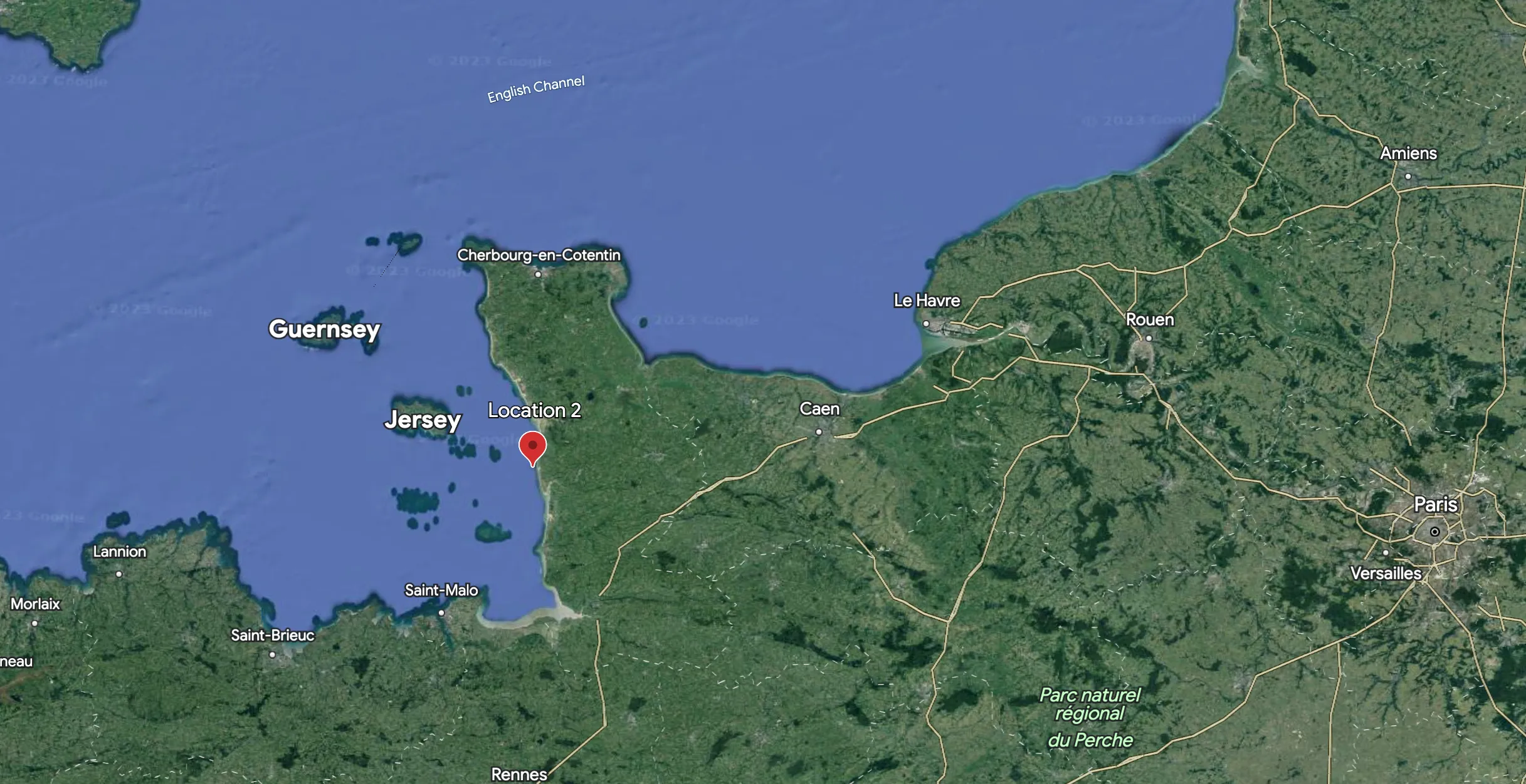
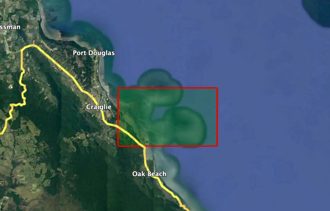
Figure 1: ‘Location 2' denotes the area of interest along the French coast (49.065780, -1.629950). This location is the second of 13 monitored sites that comprise the 26-year time series dataset (Source: Google Earth).

Oyster mortality did not appear visually correlated to any available biogeochemical data, where a considerable increase in oyster mortality during 2008–2009 was not accompanied by any noticeable change in biogeochemical parameters (Figure 2). This may be a result of the limited accuracy of the NEMO global model in a regional context, but may also suggest the presence of other external factors contributing to oyster mortality. This phenomenon was consistent amongst most sample locations and agrees with the abnormally high mortality rates in Pacific oysters observed along the French coast in the summer of 2008 that was found to be a result of an outbreak of an Ostreid herpesvirus-1 outbreak (OsHV-1) (Segarra et al., 2010). This suggests the drawbacks of purely using modelled biogeochemical data, and thus the need for diverse monitoring providers and goals to provide a comprehensive understanding of other variables such as pathogens, ecosystem biodiversity and interspecific competition that may contribute to decreased probabilities of successful restoration beyond water quality parameters.

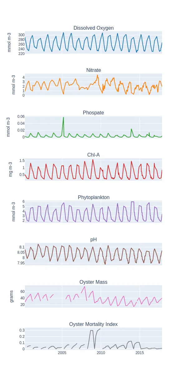
Figure 2: Biogeochemical data derived from the NEMO model as compared to the oyster mass and mortality data at Location 2 between 2000 and 2017. All parameters exhibit seasonality, with periodic peaks and troughs occurring during the summer and winter seasons. Oyster mortality showed a considerable increase between 2008–2009 which was preceded by a large increase in oyster mass.

Oyster mass was observed to spike in November 2007 prior to the increase in oyster mortality in September 2008 (Figure 3). Following this mortality event, oyster mass on average appears lower than before the event. This is consistent with a mass mortality event occurring in the Mississippi Sound, USA in 2016, whereby it was found that oyster weights did not return to levels observed before the event, and the size frequency of the population following the mortality event favoured smaller individuals (Pace et al., 2020).

Figure 3: Oyster mass and oyster mortality between 2000 and 2017 at location 2 along the French coast (Mazaleyrat et al., 2022). Both oyster mass and mortality appear seasonal, however they considerably increased in November of 2007 and September of 2008, respectively.

Whilst statistical analyses are needed to draw precise conclusions or correlations, pH is observed to decrease throughout the measured time period of 2005 to 2015 (Figure 4). This may be associated with the overall decrease in oyster mass over time observed in figure 3. Since oyster mass measured both oyster tissue and shell (Mazaleyrat et al., 2022), this decrease in pH may contribute to a change in oyster shell composition and density, thereby reducing oyster mass (Meng et al., 2018). Decreases in pH have also been associated with negative outcomes in relation to shell planting as a main component of oyster restoration efforts, where dead oyster shell is planted to initiate oyster recruitment (Waldbusser et al., 2011).

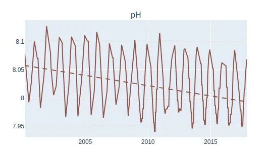
Figure 4: Despite seasonality, decreases in pH was observed at Location 2 and its surrounding areas between 2000 and 2017 (Mazaleyrat et al., 2022).

Reliance on biogeochemical models for the maintenance and protection of restored oyster reefs faces many limitations. At the moment, in situ measurements and real-time remote sensing data is predominantly used for oyster restoration projects. The NEMO model as used in this exploratory study is a global model, with limited data available for estuarine locations, the predominant environment for reef restoration projects in Australia, particularly New South Wales. The use of CSIRO’s regional model would be beneficial for further exploration of biogeochemical parameters within these Australian locations. Additionally, the NEMO model lacks fine resolution that would enable a more accurate and reliable representation of the biogeochemical properties at specific locations. However, this project was not intended as a rigorous scientific study, instead, we show that biogeochemical parameters can be derived from a global model to be used in conjunction with biological data as an important contributor to predicting the health and success of oyster restoration projects. This project was only an exploration of what could be obtained quickly with the NEMO model, and a tentative investigation into the potential correlations between environmental data and biological data derived from oyster restoration projects.

This study has been conducted using E.U. Copernicus Marine Service Information; https://doi.org/10.48670/moi-00019

About the authors —

Deepti Mallampalli and Tahlia Martignago are students at the University of Technology Sydney, where Deepti studies a Bachelor of Computer Science, majoring in Data Analytics and AI, whilst Tahlia studies a Bachelor of Science (Environmental Science) and a Bachelor of Creative Intelligence and Innovation. This project took place through the internship programs offered at UTS under the supervision and expertise of Dr Iwan Cornelius of Amentum Scientific. A big thank you is also extended to Thomas Pugh, for their expertise in developing the interface for the NEMO model that was crucial to obtaining the data we used in this study. We have been so grateful for the opportunity to receive first-hand industry experience, and have learnt so much about modelling as a tool for oceanic monitoring, and how to interpret this data with biological and industry relevance.

observing phytoplankton from space: the challenges and advantages

Author: Chloe-Marie Hawley

Date: 3 May 2023

Phytoplankton are microscopic aquatic phototrophs, ubiquitous in both marine and freshwater ecosystems, that are critical to the health and functioning of the oceans and the climate. Phytoplankton biomass is a measure for marine primary productivity; phytoplankton form the bases of all aquatic food chains and account for approximately half of the production of organic matter on Earth (Boyce et al., 2010). Additionally, phytoplankton is an important agent in the global carbon cycle; as phototrophs, phytoplankton fix carbon dioxide through photosynthesis, accounting for about 40% of the total carbon dioxide fixed naturally (Falkowski, 1994). These two important roles exemplify the ecosystem services phytoplankton provide, services that can extend to the whole planetary biogeochemical system. Consequently, variation in the ocean’s phytoplankton biomass can explain trends in the global carbon budget and possible changes in trophic level interactions, which are important to understand particularly in the face of climate change.

The distribution of phytoplankton across the oceans is driven primarily by patterns in nutrient levels. Oligotrophic regions, such as the subtropical gyres (deep blue areas, Figure 1), are nutrient poor areas that sustain low levels of phytoplankton biomass and thus low primary productivity levels. In contrast, eutrophic regions are nutrient rich and maintain high phytoplankton biomass, sometimes with frequent algal blooms when nutrients are in excess. The North Atlantic and the majority of coastal zones are eutrophic (see green areas, Figure 1). As phytoplankton biomass is tightly coupled to nutrient availability, changes, such as expansions or reductions, in these eutrophic and oligotrophic regions can predict spatial changes in phytoplankton abundances.

Figure 1: Oceanic chlorophyll concentration (proxy for phytoplankton biomass) follows the patterns of nutrient levels in the oceans: nutrient-poor oligotrophic regions show low levels of chlorophyll (blue) and nutrient-rich eutrophic regions show high levels of chlorophyll (green). (Modified image from Uitz et al., 2006).

Natural variability in phytoplankton abundance is in synchrony with seasonal change in climatic variables, notably daylight, temperature, and nutrient levels. In general, phytoplankton abundances vary over a 12-month period, in a cycle known as the spring-bloom. Like terrestrial plants, phytoplankton bloom at the onset of spring when daylight increases and nutrients, brought up the water column by storms and turbulent flows during the winter months, settle near the surface. Certain regions can instead experience a dominant 6-month period of phytoplankton abundance, blooming once in spring and once in autumn. Variability around these natural cycling patterns follows annual variation in climatic and oceanic parameters, especially sea surface temperatures. Moreover, the natural patterns are confounded by other driving forces, including human activity, anomalous weather events, and changes in trophic interactions. Partly due to the multiplicity of interactions, no global wide trend of increase or decrease in phytoplankton biomass in the past century has been robustly observed (Wernand et al., 2013). However, this is also due to the inconsistent quantitative analysis of phytoplankton biomass over sufficient spatio-temporal scales.

The importance of phytoplankton is undeniable as the primary producers of the oceans and key contributors to global carbon sequestration. So how can we better understand and monitor phytoplankton biomass at the global scale?

Phytoplankton biomass is readily derived from Earth Observation data that records several important oceanographic parameters. Satellite imagery records ocean colour which can be used to derive chlorophyll concentration in the ocean, a proxy for the phytoplankton biomass present. This is because changes in water colour are caused by a change in the composition of optically active substances, such as biological pigments. An increase in chlorophyll concentration colours the water green, and sometimes red due to the carotenoids in certain phytoplankton species. Thus, by measuring the blue, green, and red wavelengths within the ocean image, an estimate of the chlorophyll concentration can be calculated. We set out to illustrate the ease at which phytoplankton populations can be located, and observed to record change over time, using satellite observations from space.

Our methodology was simple, and while the full details of an accurate calculation are much more involved, it serves to demonstrate how quickly and easily we can start to get a sense of the global abundance of these microorganisms that are crucial for sustaining delicate marine ecosystems and maintaining Earth’s climate balance.

Planet Lab PBC’s PlanetScope satellite constellation produces comprehensive daily images of the globe at a 3m resolution. Using the surface reflectance product we were able to download pre-processed surface reflectances in 8 spectral bands for a variety of locations along the north-east coast of Australia around the Great Barrier Reef (Figure 2). Near-surface chlorophyll concentration can be calculated using empirical relationships derived from ground truth and remote sensing surface reflectances in the 440–670 nm spectral regime. Following the band difference approach established by Hu et al. (2019), we generated a measure that is proportional to chlorophyll concentration and therefore the abundance of phytoplankton, validating this measure against NASA’s publicly available chlorophyll concentration data product obtained using MODIS. MODIS measures at a 4km resolution, so the pixel values of the surface reflectance data were averaged over a 4km area for this validation. This allowed us to plot colour enhanced visuals of the same region, and observe how the abundance of these microorganisms change on short timescales. Our area of interest was a region of the Great Barrier Reef in the Coral Sea, Eastern Australia (Figure 2).

Figure 2: Area of interest along the Queensland coast. Coordinates (longitude, latitude) of top left corner are (145.486, -16.518) and bottom right is (145.584, -16.573). (Source Google Earth)

The results were as follows:

Figure 3: Distribution of phytoplankton populations on 20/09/2022 (left) and 02/10/2022 (right). Greener regions correspond to areas with more phytoplankton. Images derived from satellite imagery provided by Planet Labs PBC.

Simply, an abundance of near surface phytoplankton looks greener than the surrounding plankton-free ocean, so by comparing surface reflectance in the blue and green spectral bands, we can literally see the phytoplankton from space. This is pretty amazing.

The method is faced with many limitations, such as a lack of comparison to in situ measurements; noise in the data due to reef structures and significant changes in ocean depth; and neglect of the algorithmic complexity required to deal with many different concentrations of phytoplankton (see here for detail on the algorithms used to assemble the NASA Earth Data chlor_a product). However, this project was not intended to be a rigorous scientific study. Instead, we show that qualitative changes in phytoplankton biomass over time can be observed despite difficulties in determining accurate quantitative measurements. These observations are made in a region close to the shore, an important stepping stone to overcoming one of the biggest limitations within this field; the lack of phytoplankton data derived from satellite imagery for areas within 100km of the shoreline. In effect, PlanetScope provides satellite imagery for coastal areas that have typically been excluded, and thus is an important contributor to improving the observations, and thereby understanding, of phytoplankton biomass in coastal ecosystems.

The finer resolution of satellite imagery coupled with the development of algorithms that can distinguish between different types of phytoplankton (Xi et al., 2020) and increase the accuracy of existing algorithms, promises a leap in the improvement with which we can observe and monitor phytoplankton biomasses across time and space. This project was meant only as an exploration of what can be obtained quickly with PlanetScope data, and a primitive demonstration of the abundance of these microorganisms and how they change over time.

There has been growing concern over the anthropogenic effects on phytoplankton populations, for example, it has been shown that barge trafficking in the River Ganga, India, causes a significant decrease in plankton biomass and damage to their cell structure (Das Sarkar, 2019). The high resolution daily imaging available on PlanetScope could prove invaluable to assessing the live impact of human activity such as change in commercial shipping routes or an increase in the number of fishing vessels in any given location.

About The Authors:

Maximilian Hadley (MPhys), Joseph Phelps (MPhys) and Chloe-Marie Hawley (MBiol) are final year masters students at the University of Oxford with research interests spanning Climate Science, Earth Observation and Marine Ecology. This project took place as part of the Oxford University Micro-Internship Programme with industry participant Amentum Scientific. Under the guidance and expertise of Dr Iwan Cornelius, Managing Director of Amentum Scientific, we have learnt a great deal about how to derive important parameters from satellite imagery and how to interpret these observations with biological and ecological relevance. The data used for the project was obtained using the PlanetScope constellation of cubesats (SuperDoves) and made available via the Planet Explorer web-tool. We have all greatly appreciated the opportunity to access this relatively new platform and get first-hand experience with industry leaders. Ultimately, the outcome of our exploratory project has been to help direct the company’s use of fine-scale satellite imagery to monitor phytoplankton biomass across the Eastern Australian coastline, to flag up important limitations and their solutions, and finally to suggest possible ways to monitor the effects of human activity (such as shipping) on phytoplankton biomass within the Coral Sea, Australia.

oceanographic data at your fingertips with our new web api

Author: Iwan Cornelius

Date: 11 April 2022

The OECD predicts the value added by the Ocean Economy will reach USD 3 trillion in 2030, with a significant increase in fisheries, off-shore infrastructure, and port activities. Science, technology, and innovation play a critical role in protecting our fragile oceans from this economic development, and preserving it for future generations.

Forecasting ocean quantities such as temperature, salinity, and currents is of interest to all ocean stakeholders. Temperature affects weather phenomena such as the formation of tropical cyclones, cooling and warming of land masses, sea breezes and sea fog. Salinity is an important factor in chemistry and biochemistry of natural waters and is an important ecological factor, determining which species inhabit a given area. Salinity and temperature are both drivers of ocean circulation as they affect the density of seawater. Ocean currents are important for the study of marine debris and climate change, and are important to improving the efficiency of ocean freight.

Ocean current magnitudes (off the East coast of Australia) nowcast by the global ROTFS and accessed via our Ocean API on 2nd April 2022.

The official global Real-Time Ocean Forecast System RTOFS was developed and made available by the US National Weather Service and the US Navy. It is operated by the US National Centers for Environmental Prediction (NCEP) and provides 3D gridded data with a 24 hour time step, forecasting ahead 120 hours.

We are excited to announce the release of our new Ocean web API. The API provides machine-to-machine access to nowcast values of salinity, temperature, and currents, as predicted by the RTOFS model, for the following day.

Visit our website to try the API for free.

Please contact us if you have any questions, if other quantities (such as sea ice thickness) or greater forecast horizons are needed, or if you would like to discuss partnering opportunities.

We hope the API helps you to innovate faster and to create a safer, more sustainable, and more efficient ocean economy!

The A-team

atmosphere api update: automated retrieval of space weather indices

Author: Iwan Cornelius

Date: 10 July 2020

Figure 1: Density of the thermosphere at the altitude of the International Space Station during the geomagnetic storm of November 2018.

Satellites in Low Earth Orbit (LEO) occupy a region of Earth’s atmosphere known as the thermosphere. Even though the air is rarefied, it does result in drag forces on satellites and debris, affecting the decay of their orbits. Being able to predict the orbits of satellites and space debris is critical to safe space operations in an increasingly cluttered environment. In order to make those predictions, we need accurate models of thermospheric mass density.

The Committee on Space Research (COSPAR) is an international body that promotes scientific space research. The COSPAR International Reference Atmosphere 2012 recommends the use of two models to calculate themospheric density and composition:

1. NRLMSISE00 —developed by the US Naval Research Laboratory.
2. JB2008 — developed by Space Environment Technologies and the US Air Force Space Command.

Amentum’s Atmosphere API (accessible here) provides programmatic access to both. The nrlmsise00 and jb2008 API endpoints both calculate atmospheric density at a given altitude, latitude, longitude, date, and UTC time. The nrlmsise00 API endpoint previously required users to specify space weather indices, including:

1. The average “ap” values in the 24 hours preceding the given date,
2. F10.7 cm radio emissions for the previous day, and
3. the 81 day average of the same centered on the given date.

In response to feedback from users, we have updated the Atmosphere API to automatically retrieve space weather indices from online data sources (the US National Oceanic and Atmospheric Administration for radio flux data and GFZ German Research Centre for Geosciences for ap indices). The calculated average values are also returned in the JSON response for reference.

Figure 1 above shows the updated API in action. The global map of thermospheric density is plotted at 3 hour timestamps during the geomagnetic storm of November 2018. The diurnal variation caused by solar heating of the atmosphere (varying with time, latitude, and longitude) is apparent. The geomagnetic storm peaked around the 5th day, leading to significant increases in density that affected the orbits of satellites and debris. Note that the surge in density is pronounced at higher latitudes — caused by coupling of the magnetosphere to the solar wind (also evidenced by increased auroral activity). An excellent scientific review of thermospheric mass density, and the physical phenomena affecting it, can be found here.

The updated Atmosphere API is live and ready to use. As always, we welcome and appreciate any feedback or questions that you have.

team@amentum.space

space radiation api: on demand access to van allen belt models

Author: Iwan Cornelius

Date: 7 April 2020

A hostile radiation environment awaits any space mission. Space radiation increases the risk of cancers in humans and malfunctions in spacecraft electronics. Space radiation effects are increasingly significant, with longer duration missions to cislunar space and beyond. Moreover, the use of commercial off-the-shelf electronics that may not be resilient to radiation damage is prevalent in low cost satellites.

The environment is dominated by three sources of radiation: galactic cosmic rays (GCR), solar energetic particles (SEP), and trapped radiation. GCRs are high energy atomic nuclei that originate from outside our solar system, generated by supernovae and other phenomena. SEPs, on the other hand, are generated by our Sun during sporadic and intense solar flares. Trapped radiation comprises charged particles that are confined by the magnetic field of the Earth. Also known as Van Allen Belts (named after James Van Allen who was instrumental to their discovery) they usually consist of an inner belt of high energy protons (products of GCR interaction with the atmosphere) and an outer belt of lower energy particles (mostly electrons captured from the solar wind). A third ring between the two has also been observed [1]. Satellites in low earth orbit will traverse the inner belt when they fly over the South Atlantic ocean; craft in higher orbits or transiting to the moon or mars must endure the outer belt as well.

Source NASA https://svs.gsfc.nasa.gov/4048

Mitigating the risk of space radiation effects requires both theoretical and experimental approaches. Terrestrial-based particle accelerator facilities can bombard components and subsystems with a similar mix of radiation types and energies to ensure they are fit for purpose. However, such facilities are often prohibitively expensive or unavailable to many organizations. Theoretical studies have an important role to play. Researchers are working hard to develop and validate scientific models that can predict the space radiation environment [2]. The models are used to design radiation shielding, select components, and implement mitigation strategies such as having redundant systems or changing the state of vulnerable components in high radiation regions.

The United States Air Force Research Laboratory, in collaboration with industry partners, has developed models of Earth’s trapped radiation field. The AE9/AP9/SPM models predict the particle flux on a particular date at a particular position, or indeed for an entire mission profile.

Integrating scientific models into software systems can be challenging. Amentum Scientific develops web Application Programming Interfaces to Earth science models.

We have developed the Space Radiation API — a web API that provides on demand access to the AE9/AP9/SPM models for mission planners and engineers seeking to understand the space radiation environment. Visit our website to try the API, and please contact us if you have any questions.

https://amentum.io

Good luck and godspeed!

The A-Team

References

[1] https://www.nature.com/news/ephemeral-third-ring-of-radiation-makes-appearance-around-earth-1.12529

[2] Xapsos, Michael A., Patrick M. O’Neill, and T. Paul O’Brien. “Near-Earth space radiation models.” IEEE Transactions on Nuclear Science 60.3 (2012): 1691–1705.

Space Radiation